The traveltime-package allows to retrieve isochrones for traveltime-maps from the Traveltime Platform API directly from R. The isochrones are stored as sf-objects, ready for visualization or further processing. The isochrones display how far you can travel from a certain location within a given timeframe. Numerous modes of transport are supported.
http://docs.traveltimeplatform.com/overview/introduction
GET an API-KEY here: http://docs.traveltimeplatform.com/overview/getting-keys/
For non-commercial use the usage of the API is free up to 10’000 queries a month (max 30 queries per min). For commercial use (e.g. to integrate the API into a website) a license is needed.
devtools::install_github("tlorusso/traveltime")

# load packages
if (!require("pacman")) install.packages("pacman")
pacman::p_load(dplyr, purrr, sf, mapview, traveltime)
You can easily retrieve the isochrones with the traveltime_map function. Find a list of supported countries here: http://docs.traveltimeplatform.com/overview/supported-countries/
Querying the Traveltime-API with traveltime_map
# retrieve data via request

# The following transport modes are supported:

# "cycling"", "cycling_ferry", "driving", "driving+train", "driving_ferry", "public_transport",
# "walking", "walking+coach", "walking_bus", "walking_ferry" or "walking_train".

# how far can you go by public transport within 30 minutes?
traveltime30 <- traveltime_map(appId="YourAppId",
               apiKey="YourAPIKey",
               location=c(47.378610,8.54000),
               traveltime=1800,
               type="public_transport",
               departure="2018-11-15T08:00:00+01:00")

# ... and within 60 minutes?
traveltime60 <- traveltime_map(appId="YourAppId",
               apiKey="YourAPIKey",
               location=c(47.378610,8.54000),
               traveltime=3600,
               type="public_transport",
               departure="2018-11-15T08:00:00+01:00")
If you are interested in the opposite (from how far is location y reachable within x minutes) just use the arrival argument instead of departure.
The result of the traveltime_map-query: an sf-dataframe containing the traveltime-multipolygon as well as the request-parameters.
traveltime30

Simple feature collection with 1 feature and 6 fields
geometry type:  MULTIPOLYGON
dimension:      XY
bbox:           xmin: 8.049057 ymin: 47.16921 xmax: 8.823337 ymax: 47.52982
epsg (SRID):    4326
proj4string:    +proj=longlat +datum=WGS84 +no_defs
       lat  lng traveltime             type            departure arrival                       geometry
1 47.37861 8.54       1800 public_transport 2018-12-06T08:00:00Z      NA MULTIPOLYGON (((8.049506 47...
Taking a glimpse at the isochrones (mapview)
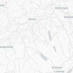
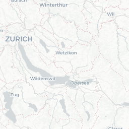
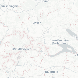
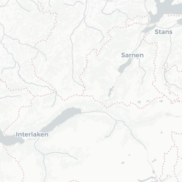
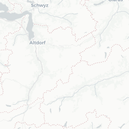
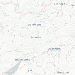
How far you can travel from Zurich Mainstation by public transport within 30 minutes or within an hour? The retrieved isochrones can be visualized with mapview to take a first glimpse.
m1 = mapview(traveltime60,  col.regions = c("grey"))
# add the second layer on top
m1 + traveltime30
Plotting a Traveltime-Map (ggmap & ggplot2)
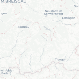
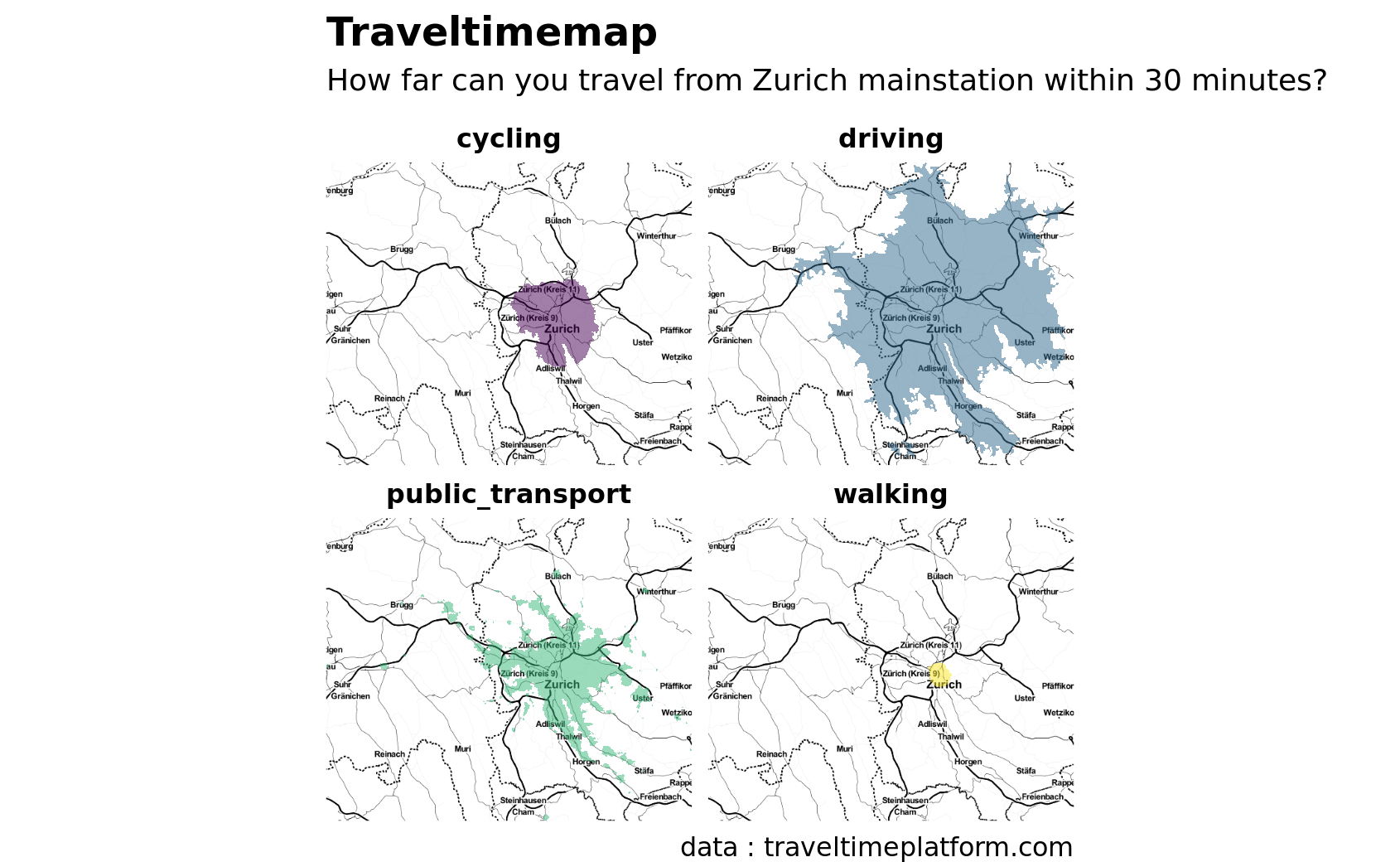
With the latest version of ggplot2, geom_sf has been introduced, which allows to plot geodata stored in dataframes with class sf very conveniently. Let’s retrieve isochrones for four different travel modes and compare how far you can go by foot, bike, car or public transport within half an hour.
# with purrr::map we can easily retrieve isochornes for different timespans


traveltimes <-c("walking","cycling","driving","public_transport") %>%
  map(.,~traveltime_map(appId="YourAppId",
                        apiKey="YourApiKey",
                        location=c(47.37787,8.54045),
                        traveltime=1800,
                        type=.x,
                        departure="2018-11-15T08:00:00+01:00") %>%
        mutate(mode=.x))

# map_dfr does not work well with sf objects (yet?) so we just..

# ... rbind the dataframes toghether via do.call
df<-do.call(rbind.data.frame, traveltimes)
library(ggmap)

#get basemap with ggmap
basemap <- get_stamenmap(bbox = unname(st_bbox(traveltimes)),maptype = "toner-hybrid")

#plot
ggmap(basemap)+
  geom_sf(data=traveltimes,inherit.aes = FALSE, aes(fill=mode), alpha=0.5,color=NA)+
  scale_fill_viridis_d()+
  theme_void()+
  coord_sf(datum = NA)+
  facet_wrap(~mode)+
  guides(fill="none")+
  theme(plot.title=element_text(face="bold"),
        plot.subtitle=element_text(size = 10, margin=margin(t=5, b = 10)),
        strip.text=element_text(face="bold",margin=margin(b = 4)))+
  labs(title="Traveltimemap", subtitle="How far can you travel from Zurich mainstation within 30 minutes?",         caption="data : traveltimeplatform.com")
#Creating an animated Map with gganimate : Rush Hour VS Night Time Drive
How far can you drive within 30min from Zurich at 7AM vs 11PM? An animated map unveils the difference in range impressively.
We can call the traveltime-API to get the isochrones for several departure-times. We could do the same for different modes of transport, locations and traveltime. With purrr::map we can pass vectors of elements to the traveltime_map- function to do so.
traveltimes <- c("2018-11-12T07:00:00+01:00","2018-11-12T23:00:00+01:00") %>%
  map(.,~traveltime_map(appId="YourAppId",
                        apiKey="YourApiKey",
                        location=c(47.378610,8.54000),
                        traveltime=1800,
                        type="driving",
                        departure=.x) %>% mutate(time=.x))

# rbind to get a dataframe
animationdf <-do.call(rbind, traveltimes)
Just with a few lines of extra code we can turn a static map into an animated one with gganimate! This works best with a single polygon-geometry. As you might notice in the case of multipolygons, the polygons break up.
#get basemap with ggmap

basemap <- get_stamenmap(bbox = unname(st_bbox(animationdf)),maptype = "toner-hybrid")

#just a few lines more to trigger gganimate!
animation <- ggmap(basemap)+
  geom_sf(data = animationdf, aes(group=type,fill=departure),inherit.aes = FALSE, alpha=0.4, colour=NA)  +
  theme_void()+
  theme(plot.title=element_text(face="bold"),
        plot.subtitle=element_text(size = 13, margin=margin(t=5, b = 10)))+
  coord_sf(datum = NA)+
  transition_states(departure, 1, 2)+
  scale_fill_manual(name="Departure time", values = c("steelblue", "darkblue"))+
  labs(title = 'How far can you drive within half an hour from Zurich mainstation?', subtitle='Departure : {closest_state}',caption="data : traveltimeplatform.com")

animation

#save the animated map as .gif
# anim_save("traveltime.gif")
To achieve a smoother transition in the case we actually get multipolygons as a result of a query, we can interpolate polygons grouped by size. However, this approach has its downside too, as some smaller polygons might ‘fly’ around. This is just ment as a quick example of what can be done with the traveltime-isochrones. There sure are much more sophisticated approaches to achieve an elegant transformation (suggestions are welcome!).
#decompose multipolygon into single polygons with the sf package
animationdf2 <- animationdf %>% sf::st_cast("POLYGON") %>%
  group_by(departure)%>%
 mutate(group=dense_rank(desc(st_area(geometry))))

# switch grouping variable
animation <- ggmap(basemap)+
  geom_sf(data = animationdf2, aes(group=group,fill=departure),inherit.aes = FALSE, alpha=0.4, colour=NA)  +
  theme_void()+
  theme(plot.title=element_text(face="bold"),
        plot.subtitle=element_text(size = 13, margin=margin(t=5, b = 10)))+
  coord_sf(datum = NA)+
  transition_states(departure, 1, 2)+
  scale_fill_manual(name="Departure time", values = c("steelblue", "darkblue"))+
  labs(title = 'How far can you drive within half an hour from Zurich mainstation?', subtitle='Departure : {closest_state}',caption="data : traveltimeplatform.com")

animation

#save the animated map as .gif
# anim_save("traveltime_size.gif")